吴恩达Machine-Learning 第六周:方法偏差与方差(bias vs variance)
一般对数据集的区分分为两种:
一种是分为两份:训练集与测试集,分别占比70%和30%。
不过这种方法使用测试集来找出最优方法,所以这组theta很可能只对测试集有很好的拟合效果,而对其他数据拟合效果就差一点。因此比较建议适用第二种数据集分类方法。
第二种:训练集、交叉验证集和测试集,分别占比60%、20%、20%。
使用这种数据集划分,首先使用训练集训练theta参数,然后使用交叉验证集选出最优的theta,最后使用测试集测试出算法准确率。
偏差与方差:
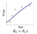
对于参数的维度d:
通常如果我们使用高纬度的参数扩展(高阶参数),对于不同的阶数,代价曲线往往如下图
对于该图
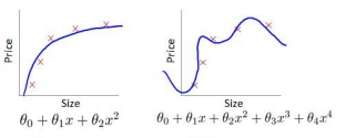
我们可以看出对于交叉验证集,前期的下降为训练结果偏差较大,往往theta不能很好地拟合曲线,因此代价会很高。而后期由于维度过高,theta对训练数据过拟合,又没有办法很好地拟合交叉训练集,因此对于交叉验证集的代价又有显著的上升。
这时候我们一般取交叉验证集中最低点的d,作为最优参数。
对于正则化lambda的选择:
和上面一样,只不过较大的正则化参数往往对代价的影响成正相关。
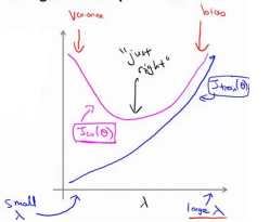
在较小的lambda的情况下(比如极端的0,这时不进行正则化),往往很容易对训练数据集过拟合,因此对于交叉验证集的代价可能会很高,产生高方差。
而在较大的lambda的情况下,又会产生欠拟合,即高偏差,这是训练集和交叉验证集的代价都会上涨。
这时候我们一般也取交叉验证集中最低点的lambda作为最优参数。
学习曲线:
学习曲线用来判断一个学习算法是否处于偏差、方差问题。
学习曲线是学习算法的一个很好的合理检验。
学习曲线是将训练集误差和交叉验证集作为训练实例数量的函数绘制的图标。
如下图:
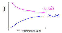
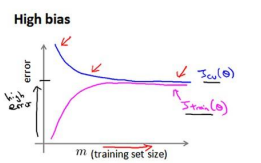
下图是高偏差情况下的代价图,对于这种欠拟合的情况下,盲目的增加训练数据量是没有什么明显作用的,往往需要减小lambda(即减少正则化强度)或者增加theta的维度,来增强theta对数据的拟合:
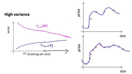
下面是高方差的情况下的代价图,而这种情况,增加训练数据量可以取得较好的结果:
下面针对具体的例子进行举例:
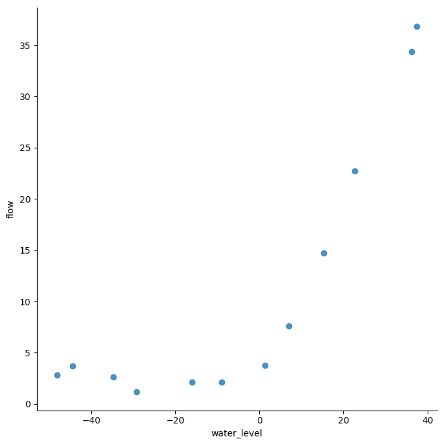
数据预览:
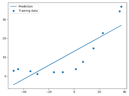
线性回归设置后的分界线:
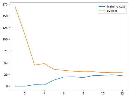
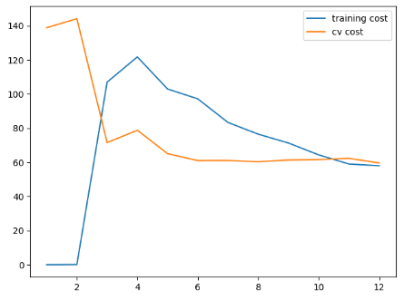
学习曲线:
不同训练集长度对训练代价以及交叉验证集代价产生的影响,可以看到这个模型并没有很好地拟合训练数据(最终两条曲线在25附近的高代价附近靠近,高偏差,有一点欠拟合):
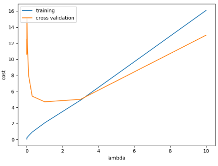
对lambda的选择:
不同lambda下训练代价和交叉校验代价的变化,可以看到大概在1附近取到最低:
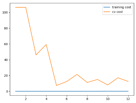
lambda = 0,训练代价低的不真实,过拟合:
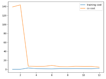
lambda = 1,训练成本有一点上升,我们假设有一点不是那么过拟合(和0比):
lambda = 100,,过多的正则化:
代码如下:
# -*- coding:utf-8 -*-
import numpy as np
import scipy.io as sio
import scipy.optimize as opt
import pandas as pd
import matplotlib.pyplot as plt
import seaborn as sns
def load_data():
    """
    文件读取
    :return:
    """
    d = sio.loadmat('./data/ex5data1.mat')
    return map(np.ravel, [d['X'], d['y'], d['Xval'], d['yval'], d['Xtest'], d['ytest']])
# 读取数据与画出初始数据图
X, y, Xval, yval, Xtest, ytest = load_data()
df = pd.DataFrame({'water_level': X, 'flow': y})
sns.lmplot('water_level', 'flow', data=df, fit_reg=False, size=7)
plt.show()
# 对X、Xval、Xtest添加Ones偏置列
X, Xval, Xtest = [np.insert(x.reshape(x.shape[0], 1), 0, np.ones(x.shape[0]), axis=1) for x in (X, Xval, Xtest)]
def cost(theta, X, y):
    """
    计算代价(平方差)
    :param theta:
    :param X:
    :param y:
    :return:
    """
    m = X.shape[0]
    inner = X @ theta - y  # R(m*1)
    # 1*m @ m*1 = 1*1 in matrix multiplication
    # but you know numpy didn't do transpose in 1d array, so here is just a
    # vector inner product to itselves
    square_sum = inner.T @ inner
    cost = square_sum / (2 * m)
    return cost
theta = np.ones(X.shape[1])
# 303.951525554
print(cost(theta, X, y))
def gradient(theta, X, y):
    """
    下降算法
    :param theta:
    :param X:
    :param y:
    :return:
    """
    m = X.shape[0]
    inner = X.T @ (X @ theta - y)  # (m,n).T @ (m, 1) -> (n, 1)
    return inner / m
# [ -15.30301567  598.16741084]
print(gradient(theta, X, y))
def regularized_gradient(theta, X, y, l=1):
    """
    正则化梯度下降
    :param theta:
    :param X:
    :param y:
    :param l:
    :return:
    """
    m = X.shape[0]
    # 不惩罚第一项
    regularized_term = theta.copy()  # same shape as theta
    regularized_term[0] = 0  # don't regularize intercept theta
    regularized_term = (l / m) * regularized_term
    return gradient(theta, X, y) + regularized_term
# [ -15.30301567  598.16741084]
print(regularized_gradient(theta, X, y))
def linear_regression_np(X, y, l=1):
    """
    线性回归
    linear regression
    args:
        X: feature matrix, (m, n+1) # with incercept x0=1
        y: target vector, (m, )
        l: lambda constant for regularization
    return: trained parameters
    """
    # init theta
    theta = np.ones(X.shape[1])
    # train it
    res = opt.minimize(fun=regularized_cost,
                       x0=theta,
                       args=(X, y, l),
                       method='TNC',
                       jac=regularized_gradient,
                       options={'disp': True})
    return res
def regularized_cost(theta, X, y, l=1):
    """
    正则化代价函数
    :param theta:
    :param X:
    :param y:
    :param l:
    :return:
    """
    # 不惩罚第一项
    m = X.shape[0]
    regularized_term = (l / (2 * m)) * np.power(theta[1:], 2).sum()
    return cost(theta, X, y) + regularized_term
theta = np.ones(X.shape[0])
# 获得训练好的theta [ 13.08790362   0.36777923]
final_theta = linear_regression_np(X, y, l=0).get('x')
b = final_theta[0]  # intercept
m = final_theta[1]  # slope
# 画出训练好的图像
plt.scatter(X[:, 1], y, label="Training data")
plt.plot(X[:, 1], X[:, 1] * m + b, label="Prediction")
plt.legend(loc=2)
plt.show()
training_cost, cv_cost = [], []
m = X.shape[0]
# 不同训练集大小对代价的变化产生的影响
for i in range(1, m + 1):
    #     print('i={}'.format(i))
    res = linear_regression_np(X[:i, :], y[:i], l=0)
    tc = regularized_cost(res.x, X[:i, :], y[:i], l=0)
    cv = regularized_cost(res.x, Xval, yval, l=0)
    #     print('tc={}, cv={}'.format(tc, cv))
    training_cost.append(tc)
    cv_cost.append(cv)
# 绘制不同训练集大小下的代价变化图
plt.plot(np.arange(1, m + 1), training_cost, label='training cost')
plt.plot(np.arange(1, m + 1), cv_cost, label='cv cost')
plt.legend(loc=1)
plt.show()
def prepare_poly_data(*args, power):
    """
    args: keep feeding in X, Xval, or Xtest
        will return in the same order
    """
    def prepare(x):
        # expand feature
        # 特征扩展
        df = poly_features(x, power=power)
        # normalization
        # 标准化数据
        ndarr = normalize_feature(df).as_matrix()
        # add intercept term
        # 增加Ones偏置项
        return np.insert(ndarr, 0, np.ones(ndarr.shape[0]), axis=1)
    return [prepare(x) for x in args]
def poly_features(x, power, as_ndarray=False):
    """
    返回x的高阶
    :param x:
    :param power:
    :param as_ndarray:
    :return:
    """
    data = {'f{}'.format(i): np.power(x, i) for i in range(1, power + 1)}
    df = pd.DataFrame(data)
    return df.as_matrix() if as_ndarray else df
X, y, Xval, yval, Xtest, ytest = load_data()
poly_features(X, power=3)
def normalize_feature(df):
    """Applies function along input axis(default 0) of DataFrame."""
    """
    lambda表达式和def很像,只不过是一个轻量级的def
    lambda后面的变量为参数,多餐用逗号隔开。
    紧接着为表达式,用来执行对参数的相关操作。
    如下面的lambda参数等价于
    def xxx(column):
        (column - column.mean()) / column.std()
    也就是执行数据的标准化的动作
    """
    return df.apply(lambda column: (column - column.mean()) / column.std())
X_poly, Xval_poly, Xtest_poly = prepare_poly_data(X, Xval, Xtest, power=8)
print(X_poly[:3, :])
def plot_learning_curve(X, y, Xval, yval, l=0):
    """
    学习曲线
    :param X:
    :param y:
    :param Xval:
    :param yval:
    :param l:
    :return:
    """
    training_cost, cv_cost = [], []
    m = X.shape[0]
    # 不同训练集大小下的学习代价变化
    for i in range(1, m + 1):
        # regularization applies here for fitting parameters
        res = linear_regression_np(X[:i, :], y[:i], l=l)
        # remember, when you compute the cost here, you are computing
        # non-regularized cost. Regularization is used to fit parameters only
        # 记住,当你在这计算代价时,不要使用正则计算。正则计算只用来寻找参数
        tc = cost(res.x, X[:i, :], y[:i])
        cv = cost(res.x, Xval, yval)
        training_cost.append(tc)
        cv_cost.append(cv)
    plt.plot(np.arange(1, m + 1), training_cost, label='training cost')
    plt.plot(np.arange(1, m + 1), cv_cost, label='cv cost')
    plt.legend(loc=1)
# 绘制三种不同lambda对用的图像
plot_learning_curve(X_poly, y, Xval_poly, yval, l=0)
plt.show()
plot_learning_curve(X_poly, y, Xval_poly, yval, l=1)
plt.show()
plot_learning_curve(X_poly, y, Xval_poly, yval, l=100)
plt.show()
# 设置了几种lambda的值
l_candidate = [0, 0.001, 0.003, 0.01, 0.03, 0.1, 0.3, 1, 3, 10]
training_cost, cv_cost = [], []
# 对每一种lambda进行计算并且画图
for l in l_candidate:
    res = linear_regression_np(X_poly, y, l)
    tc = cost(res.x, X_poly, y)
    cv = cost(res.x, Xval_poly, yval)
    training_cost.append(tc)
    cv_cost.append(cv)
plt.plot(l_candidate, training_cost, label='training')
plt.plot(l_candidate, cv_cost, label='cross validation')
plt.legend(loc=2)
plt.xlabel('lambda')
plt.ylabel('cost')
plt.show()
# best cv I got from all those candidates
print(l_candidate[np.argmin(cv_cost)])
# use test data to compute the cost
for l in l_candidate:
    theta = linear_regression_np(X_poly, y, l).x
    print('test cost(l={}) = {}'.format(l, cost(theta, Xtest_poly, ytest)))
0 条评论