【吴恩达机器学习】异常检测算法

吴恩达Machine-Learning 第九周：异常检测算法（anomaly detection）

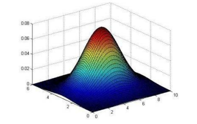
异常检测算法主要用来监测数值中的异常值，通过高斯分布，将数据映射在如下三维或者二维上，然后选择出异常值。

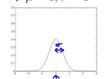
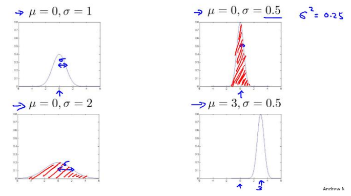
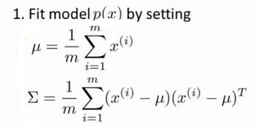
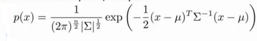
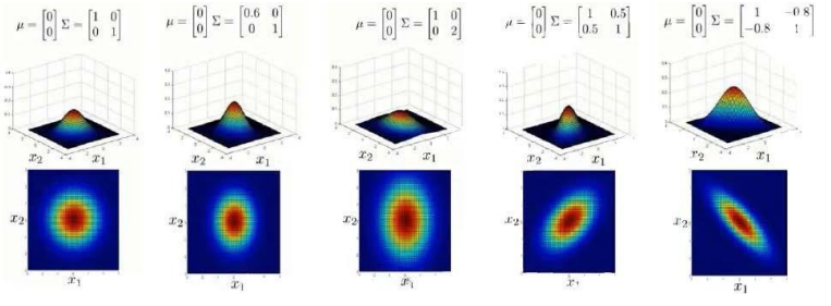
对于普通的高斯函数，我们可以通过修改高斯函数的参数来使高斯函数可以更好的拟合数据：

而这两个参数，我们可以通过下式解出：

然后通过下式，就可以将数据在高斯函数中的映射获得：

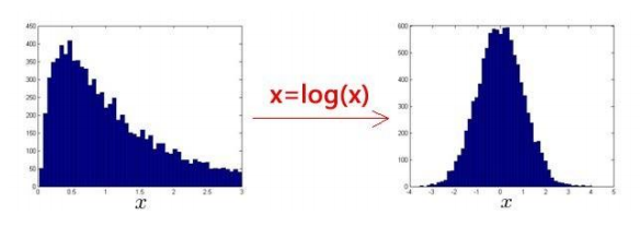
那么对于一些数据没有明显的满足高斯分布，例如下图，我们可以通过一些数学变化让它满足高斯分布

同时，我们发现 有一些数据并不是服从“水平”或者“竖直”的高斯分布，如下如蓝线，很明显能对数据更好的拟合，

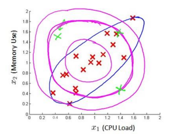
因此我们这里多了一组参数 ，可以对高斯函数的分布做出影响，也就是多元高斯函数。

而对于映射之后的值要多小才被认为是异常，我们通过下式计算：

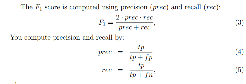
其中：

• tp means true positives：是异常值，并且我们的模型预测成异常值了，即真的异常值。
• fp means false positives：是正常值，但模型把它预测成异常值，即假的异常值。
• fn means false negatives：是异常值，但是模型把它预测成正常值，即假的正常值。

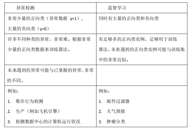
到这里我们异常检测算法的原理就基本讲完了，那么同样是“分类”问题，我们怎么选择异常检测算法与其他监督学习算法呢？

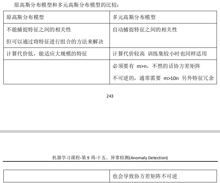
那么对于异常检测算法，我们又什么时候选择高斯分布，什么时候选择多元的高斯分布呢？

下面是代码讲解：

首先读取数据：

mat = loadmat('data/ex8data1.mat')
# dict_keys(['__header__', '__version__', '__globals__', 'X', 'Xval', 'yval'])
print(mat.keys())
X = mat['X']
Xval, yval = mat['Xval'], mat['yval']
# ((307, 2), (307, 2), (307, 1))
print(X.shape, Xval.shape, yval.shape)

将点添加进绘图中方法：

def plot_data():
    """
    绘制数据样式，第一次输出
    :return:
    """
    plt.figure(figsize=(8, 5))
    # 训练集
    plt.plot(X[:, 0], X[:, 1], 'bx')
    # 验证集
    # plt.scatter(Xval[:,0], Xval[:,1], c=yval.flatten(), marker='x', cmap='rainbow')

获取当前数据的高斯函数模型参数：

def getGaussianParams(X, useMultivariate):
    """
    获取高斯参数
    :param X: data
    :param useMultivariate: 是否使用多维高斯函数
    :return: mu和参数
    """
    # 求平均值，mu
    mu = X.mean(axis=0)
    if useMultivariate:
        # 多维高斯参数计算方法  有四个参数 2*2
        sigma2 = ((X - mu).T @ (X - mu)) / len(X)
    else:
        # 样本方差 只有两个参数
        sigma2 = X.var(axis=0, ddof=0)
    return mu, sigma2

将数据在高斯模型上的映射返回：

def gaussian(X, mu, sigma2):
    '''
    mu, sigma2参数已经决定了一个高斯分布模型
    因为原始模型就是多元高斯模型在sigma2上是对角矩阵而已，所以如下：
    If Sigma2 is a matrix, it is treated as the covariance matrix.
    If Sigma2 is a vector, it is treated as the sigma^2 values of the variances
    in each dimension (a diagonal covariance matrix)
    output:
        一个(m, )维向量，包含每个样本的概率值。
    '''
    m, n = X.shape
    # ndim返回的是数组的维度
    if np.ndim(sigma2) == 1:
        # diag：array是一个1维数组时，结果形成一个以一维数组为对角线元素的矩阵
        #       array是一个二维矩阵时，结果输出矩阵的对角线元素
        # 这里输出了对角线矩阵
        sigma2 = np.diag(sigma2)
    # 计算参数
    norm = 1. / (np.power((2 * np.pi), n / 2) * np.sqrt(np.linalg.det(sigma2)))
    exp = np.zeros((m, 1))
    for row in range(m):
        xrow = X[row]
        exp[row] = np.exp(-0.5 * ((xrow - mu).T).dot(np.linalg.inv(sigma2)).dot(xrow - mu))
    return norm * exp

绘制高斯函数图像：

def plotContours(mu, sigma2):
    """
    画出高斯概率分布的图，在三维中是一个上凸的曲面。投影到平面上则是一圈圈的等高线。
    """
    # 计算点的间隔
    delta = .3  # 注意delta不能太小！！！否则会生成太多的数据，导致矩阵相乘会出现内存错误。
    x = np.arange(0, 30, delta)
    y = np.arange(0, 30, delta)
    # 这部分要转化为X形式的坐标矩阵，也就是一列是横坐标，一列是纵坐标，
    # 然后才能传入gaussian中求解得到每个点的概率值
    # meshgrid 将数据转换为坐标形式
    xx, yy = np.meshgrid(x, y)
    # 是按行连接两个矩阵，就是把两矩阵左右相加，要求行数相等
    points = np.c_[xx.ravel(), yy.ravel()]  # 按列合并，一列横坐标，一列纵坐标
    z = gaussian(points, mu, sigma2)
    z = z.reshape(xx.shape)  # 这步骤不能忘
    # 这个levels是作业里面给的参考,或者通过求解的概率推出来。
    cont_levels = [10 ** h for h in range(-20, 0, 3)]
    plt.contour(xx, yy, z, cont_levels)
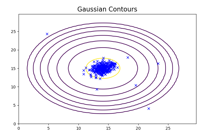
    plt.title('Gaussian Contours', fontsize=16)

我们首先看一下正常的高斯函数分布：

plot_data()
useMV = False
plotContours(*getGaussianParams(X, useMV))
plt.show()

如下图：

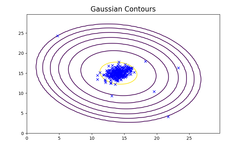
绘制多元高斯函数分布：

plot_data()
useMV = True
plotContours(*getGaussianParams(X, useMV))
plt.show()

如下图，可以看到整个高斯函数进行了偏转

选择最优阈值：

def selectThreshold(yval, pval):
    """
    选择合适的阈值，即多小的值应该被判断为异常
    :param yval:
    :param pval:
    :return:
    """

    def computeF1(yval, pval):
        m = len(yval)
        tp = float(len([i for i in range(m) if pval[i] and yval[i]]))
        fp = float(len([i for i in range(m) if pval[i] and not yval[i]]))
        fn = float(len([i for i in range(m) if not pval[i] and yval[i]]))
        prec = tp / (tp + fp) if (tp + fp) else 0
        rec = tp / (tp + fn) if (tp + fn) else 0
        F1 = 2 * prec * rec / (prec + rec) if (prec + rec) else 0
        return F1

    # 数据分割 1000份
    epsilons = np.linspace(min(pval), max(pval), 1000)
    bestF1, bestEpsilon = 0, 0
    for e in epsilons:
        pval_ = pval < e
        thisF1 = computeF1(yval, pval_)
        if thisF1 > bestF1:
            bestF1 = thisF1
            bestEpsilon = e

    return bestF1, bestEpsilon

然后我们使用验证数据进行计算：

# 获取mu 和sigma
mu, sigma2 = getGaussianParams(X, useMultivariate=True)
# 利用mu和sigma确定高斯函数（使用验证集）
pval = gaussian(Xval, mu, sigma2)
# 确定最佳参数
bestF1, bestEpsilon = selectThreshold(yval, pval)

这里我们找到了最佳参数之后，和训练数据算出的高斯函数进行对比：

y = gaussian(X, mu, sigma2)  # X的概率

找到离群点：

xx = np.array([X[i] for i in range(len(y)) if y[i] < bestEpsilon])
print(xx)  # 离群点

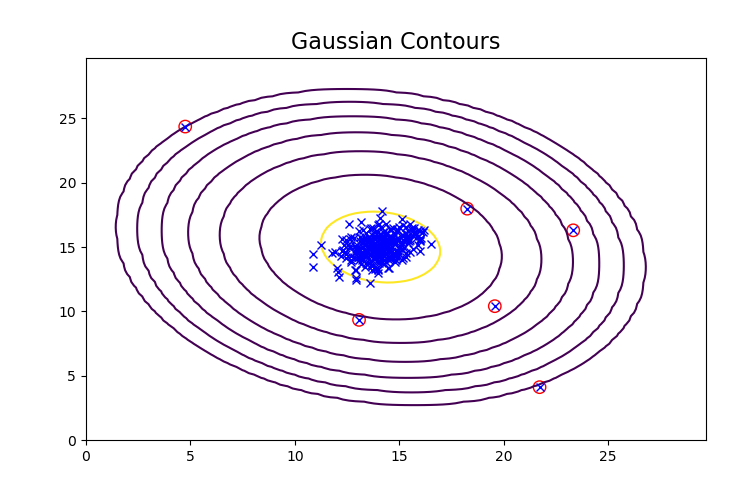
画图：

plot_data()
plotContours(mu, sigma2)
plt.scatter(xx[:, 0], xx[:, 1], s=80, facecolors='none', edgecolors='r')
plt.show()

可以看出，离群点（异常点）已经被标出：

整理后的代码：

# -*- coding:utf-8 -*-

import numpy as np
from scipy.io import loadmat
import matplotlib.pyplot as plt


def load_data():
    """
    读取数据
    :return:
    """
    mat = loadmat('data/ex8data1.mat')
    X = mat['X']
    Xval, yval = mat['Xval'], mat['yval']
    return X, Xval, yval


def get_gaussian_garams(X, useMultivariate=False):
    """
    确定高斯模型参数
    :param X: 数据
    :param useMultivariate: 是否使用多元高斯模型
    :return: 高斯参数的mu和sigma^2
    """
    mu = X.mean(axis=0)
    if useMultivariate:
        sigma2 = ((X - mu).T @ (X - mu)) / len(X)
    else:
        sigma2 = X.var(axis=0, ddof=0)
    return mu, sigma2


def gaussian(X, mu, sigma2):
    """
    获取数据通过高斯模型之后的映射
    :param X:
    :param mu:
    :param sigma2:
    :return:
    """
    m, n = X.shape
    # 如果sigma2是一维的，转换多维方便计算
    if np.ndim(sigma2) == 1:
        sigma2 = np.diag(sigma2)
    # 计算公式
    norm = 1. / (np.power((2 * np.pi), n / 2) * np.sqrt(np.linalg.det(sigma2)))
    exp = np.zeros((m, 1))
    for row in range(m):
        xrow = X[row]
        exp[row] = np.exp(-0.5 * ((xrow - mu).T).dot(np.linalg.inv(sigma2)).dot(xrow - mu))
    return norm * exp


def select_threshold(yval, pval):
    """
    选择一个合适的阈值作为异常数据的检测边界
    :param yval: 数据结果（key）
    :param pval: 通过高斯映射后的值
    :return:
    """

    def computeF1(yval, pval):
        """
        计算F1
        :param yval:
        :param pval:
        :return:
        """
        m = len(yval)
        tp = float(len([i for i in range(m) if pval[i] and yval[i]]))
        fp = float(len([i for i in range(m) if pval[i] and not yval[i]]))
        fn = float(len([i for i in range(m) if not pval[i] and yval[i]]))
        prec = tp / (tp + fp) if (tp + fp) else 0
        rec = tp / (tp + fn) if (tp + fn) else 0
        F1 = 2 * prec * rec / (prec + rec) if (prec + rec) else 0
        return F1

    # 分割数据
    epslions = np.linspace(min(pval), max(pval), 1000)
    bestF1, bestEpslion = 0, 0
    # 寻找一个最合适的点，来作为最佳的阈值
    for e in epslions:
        _pvel = pval < e
        thisF1 = computeF1(yval, _pvel)
        if thisF1 > bestF1:
            bestF1 = thisF1
            bestEpslion = e
    return bestF1, bestEpslion


def plot_data(X):
    """
    绘制数据点，由于需要多次绘制，使用方法简化流程
    :return:
    """
    plt.figure(figsize=(8, 5))
    plt.plot(X[:, 0], X[:, 1], 'bx')


def plot_contours(mu, sigma2):
    """
    画出高斯分布图
    :param mu:
    :param sigma2:
    :return:
    """
    delta = 0.3
    # 分别在0，30中间均分出x y
    x = np.arange(0, 30, delta)
    y = np.arange(0, 30, delta)
    # 将x y转换为坐标
    xx, yy = np.meshgrid(x, y)
    points = np.c_[xx.ravel(), yy.ravel()]
    z = gaussian(points, mu, sigma2)
    z = z.reshape(xx.shape)
    cont_levels = [10 ** h for h in range(-20, 0, 3)]
    plt.contour(xx, yy, z, cont_levels)
    plt.title('Gaussian Contours', fontsize=16)


X, Xval, yval = load_data()
mu, sigma2 = get_gaussian_garams(X, useMultivariate=True)
pval = gaussian(Xval, mu, sigma2)
bestF1, bestEpsilon = select_threshold(yval, pval)

y = gaussian(X, mu, sigma2)  # X的概率
# 计算离群点
xx = np.array([X[i] for i in range(len(y)) if y[i] < bestEpsilon])
plot_data(X)
plot_contours(mu, sigma2)
# 绘制离群点
plt.scatter(xx[:, 0], xx[:, 1], s=80, facecolors='none', edgecolors='r')
plt.show()
print()